> ## Documentation Index
> Fetch the complete documentation index at: https://nixtla-docs-feat-simulate-and-explain.mintlify.site/llms.txt
> Use this file to discover all available pages before exploring further.
# Advanced explanations
> Compare historical relationship analyses, forecast allocations, and stability across time.
This guide is for users who want more control over how historical relationships
are measured or used in a forecast explanation.
Start with the customer-facing guides if your question is simply:
* [Why did TimeGPT make this
forecast?](/forecasting/exogenous-variables/interpretability_with_shap)
* [What is the forecast sensitive
to?](/forecasting/explanation/intervention)
* [Which signals have been useful
historically?](/forecasting/exogenous-variables/causal-explanations)
The examples below continue with the same retail `df` and future `X_df` from
those guides.
## Compare historical relationship analyses
`explain()` provides two complementary analyses:
| Analysis | Useful when |
| ---------------- | ------------------------------------------------------------------ |
| Granger | You want a fast first pass focused on linear, lagged relationships |
| Transfer entropy | You expect nonlinear or more complex lagged relationships |
Run both on the same data:
```python theme={null}
granger_signals = nixtla_client.explain(
df=df,
features=["price", "promotion", "temperature"],
method="granger",
)
entropy_signals = nixtla_client.explain(
df=df,
features=["price", "promotion", "temperature"],
method="transfer_entropy",
)
```
| Feature | Granger | Transfer entropy |
| ----------- | ------: | ---------------: |
| Price | 0.000 | 0.502 |
| Promotion | 0.863 | 0.046 |
| Temperature | 0.137 | 0.452 |
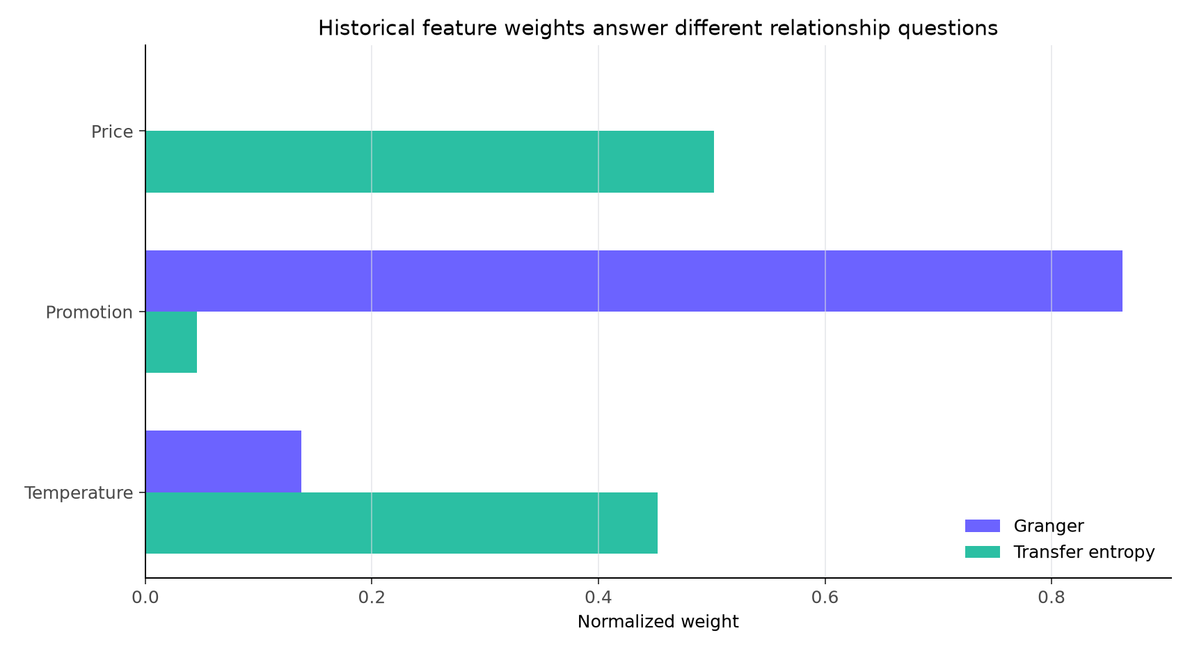 The linear analysis emphasizes promotion. Transfer entropy finds more
historical information in price and temperature. The useful question is not
which analysis “wins,” but which relationship matches what you are
investigating.
## Allocate a forecast using historical relationships
TimeGPT can also use those historical weights to divide the movement of a
forecast around its starting value:
`"granger"` and `"transfer_entropy"` appear in two different places. As the
`method` argument to `explain()` (above) they screen historical relationships
without a forecast. As `feature_contributions_type` in `forecast()` (below) they
use those same relationship measures to allocate a forecast. Same names, two
mechanisms.
```python theme={null}
forecast = nixtla_client.forecast(
df=df,
X_df=X_df,
h=14,
freq="D",
model="timegpt-2.1",
feature_contributions=True,
feature_contributions_type="granger",
)
granger_contributions = nixtla_client.feature_contributions.copy()
forecast = nixtla_client.forecast(
df=df,
X_df=X_df,
h=14,
freq="D",
model="timegpt-2.1",
feature_contributions=True,
feature_contributions_type="transfer_entropy",
)
entropy_contributions = nixtla_client.feature_contributions.copy()
```
For the first promotion day, both views explain the same 92.01-unit forecast:
| Input | Granger-weighted | Transfer-entropy-weighted |
| ----------- | ---------------: | ------------------------: |
| Price | 0.00 | 4.33 |
| Promotion | 7.43 | 0.39 |
| Temperature | 1.18 | 3.90 |
The linear analysis emphasizes promotion. Transfer entropy finds more
historical information in price and temperature. The useful question is not
which analysis “wins,” but which relationship matches what you are
investigating.
## Allocate a forecast using historical relationships
TimeGPT can also use those historical weights to divide the movement of a
forecast around its starting value:
`"granger"` and `"transfer_entropy"` appear in two different places. As the
`method` argument to `explain()` (above) they screen historical relationships
without a forecast. As `feature_contributions_type` in `forecast()` (below) they
use those same relationship measures to allocate a forecast. Same names, two
mechanisms.
```python theme={null}
forecast = nixtla_client.forecast(
df=df,
X_df=X_df,
h=14,
freq="D",
model="timegpt-2.1",
feature_contributions=True,
feature_contributions_type="granger",
)
granger_contributions = nixtla_client.feature_contributions.copy()
forecast = nixtla_client.forecast(
df=df,
X_df=X_df,
h=14,
freq="D",
model="timegpt-2.1",
feature_contributions=True,
feature_contributions_type="transfer_entropy",
)
entropy_contributions = nixtla_client.feature_contributions.copy()
```
For the first promotion day, both views explain the same 92.01-unit forecast:
| Input | Granger-weighted | Transfer-entropy-weighted |
| ----------- | ---------------: | ------------------------: |
| Price | 0.00 | 4.33 |
| Promotion | 7.43 | 0.39 |
| Temperature | 1.18 | 3.90 |
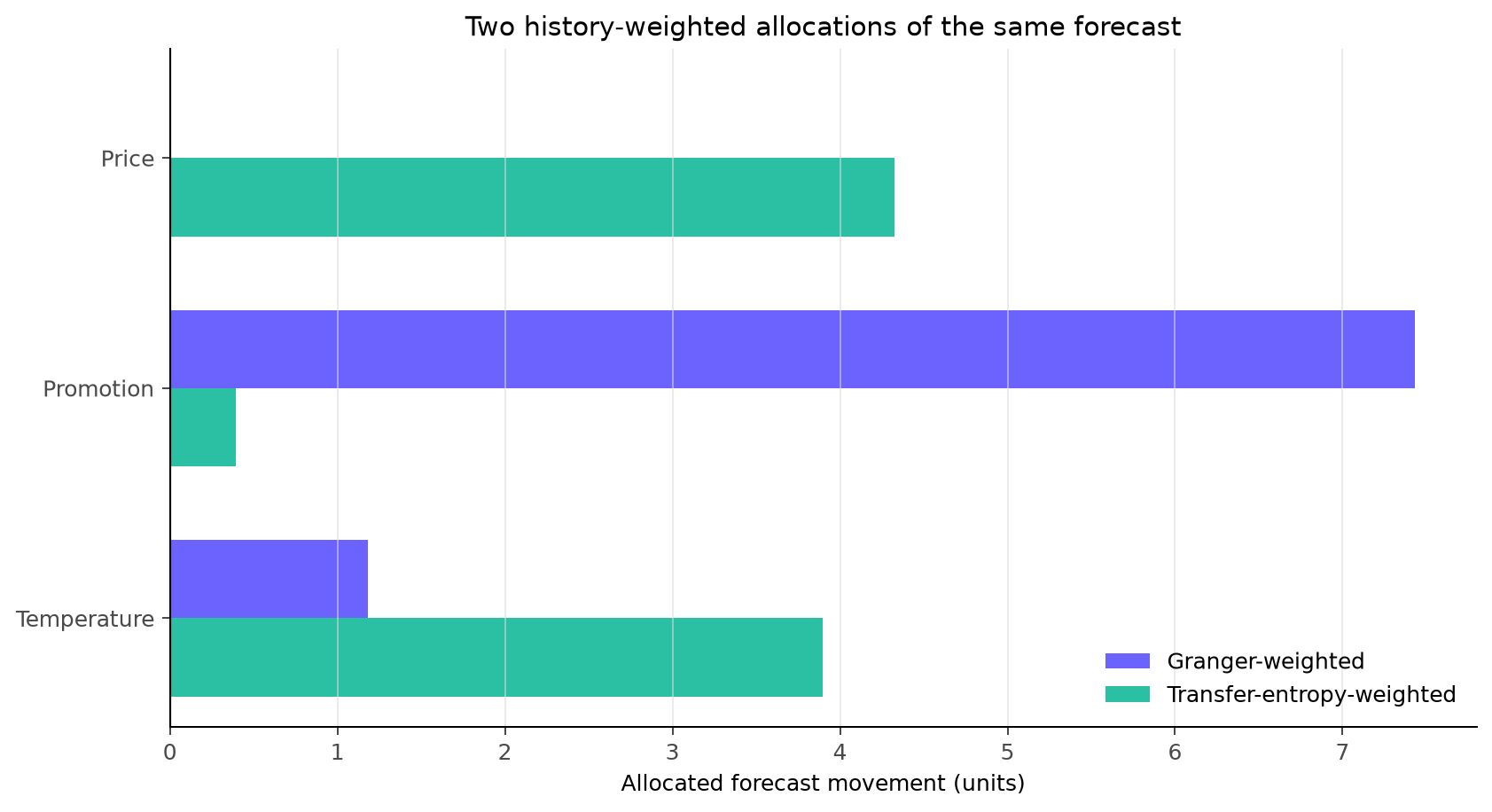 Use these views when you specifically want a forecast allocation grounded in a
selected historical relationship analysis. Use SHAP when you want the standard
prediction-level explanation.
## Check whether a ranking is stable
A feature ranking can change when the historical window changes. Re-running the
analysis over adjacent windows helps reveal persistent and temporary signals:
```python theme={null}
window_results = []
for end in range(185, len(df) + 1, 30):
window = df.iloc[end - 180 : end]
for analysis in ["granger", "transfer_entropy"]:
result = nixtla_client.explain(
window,
features=["price", "promotion", "temperature"],
method=analysis,
).assign(
analysis=analysis,
window_end=window["ds"].max(),
)
window_results.append(result)
weight_history = pd.concat(window_results, ignore_index=True)
```
Use these views when you specifically want a forecast allocation grounded in a
selected historical relationship analysis. Use SHAP when you want the standard
prediction-level explanation.
## Check whether a ranking is stable
A feature ranking can change when the historical window changes. Re-running the
analysis over adjacent windows helps reveal persistent and temporary signals:
```python theme={null}
window_results = []
for end in range(185, len(df) + 1, 30):
window = df.iloc[end - 180 : end]
for analysis in ["granger", "transfer_entropy"]:
result = nixtla_client.explain(
window,
features=["price", "promotion", "temperature"],
method=analysis,
).assign(
analysis=analysis,
window_end=window["ds"].max(),
)
window_results.append(result)
weight_history = pd.concat(window_results, ignore_index=True)
```
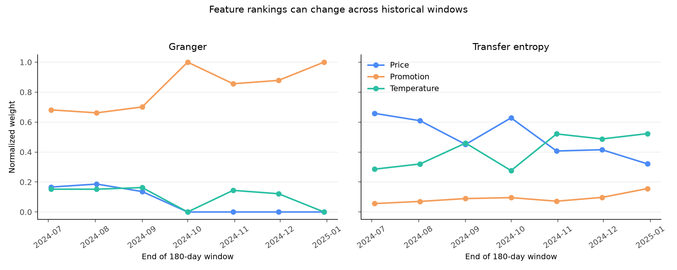 Stable rankings are easier to use operationally. A changing ranking is useful
information too: it can point to seasonality, a business shift, or a data issue
worth investigating.
## Practical details
Historical `explain()` weights are nonnegative and add to one.
Granger-weighted and transfer-entropy-weighted forecast contributions add
to `TimeGPT` together with `base_value`. Intervention contributions are
calculated one input at a time and need not add up to the forecast.
List categorical columns in `categorical_exog_list`. Historical
relationship analyses encode categories consistently before measuring
lagged relationships. Treat the result as a ranking rather than a numeric
distance between category labels.
For any `feature_contributions_type` other than `"shapley"`, categorical
features cannot be combined with `hist_exog_list` when the request also
covers historical timestamps, that is `forecast(..., add_history=True)`. The
historical/future column mapping cannot be represented faithfully once the
categorical columns are split out, so the request is rejected rather than
returning a silently wrong explanation. Either keep the exogenous features
all-numeric, drop `hist_exog_list`, or use `"shapley"`. A plain
`forecast()` call is unaffected and supports this combination.
A request supports up to 75 explained features and 1,000,000 historical
feature-observations. Transfer entropy generally takes more computation
than Granger analysis.
If an analysis cannot distinguish the selected features, `explain()` returns
equal weights. This can happen with short series, constant values, or a
historical window that contains little predictive information.
Advanced explanations are most useful when the analysis question is explicit.
Record the selected analysis and historical window alongside any result you
share.
Stable rankings are easier to use operationally. A changing ranking is useful
information too: it can point to seasonality, a business shift, or a data issue
worth investigating.
## Practical details
Historical `explain()` weights are nonnegative and add to one.
Granger-weighted and transfer-entropy-weighted forecast contributions add
to `TimeGPT` together with `base_value`. Intervention contributions are
calculated one input at a time and need not add up to the forecast.
List categorical columns in `categorical_exog_list`. Historical
relationship analyses encode categories consistently before measuring
lagged relationships. Treat the result as a ranking rather than a numeric
distance between category labels.
For any `feature_contributions_type` other than `"shapley"`, categorical
features cannot be combined with `hist_exog_list` when the request also
covers historical timestamps, that is `forecast(..., add_history=True)`. The
historical/future column mapping cannot be represented faithfully once the
categorical columns are split out, so the request is rejected rather than
returning a silently wrong explanation. Either keep the exogenous features
all-numeric, drop `hist_exog_list`, or use `"shapley"`. A plain
`forecast()` call is unaffected and supports this combination.
A request supports up to 75 explained features and 1,000,000 historical
feature-observations. Transfer entropy generally takes more computation
than Granger analysis.
If an analysis cannot distinguish the selected features, `explain()` returns
equal weights. This can happen with short series, constant values, or a
historical window that contains little predictive information.
Advanced explanations are most useful when the analysis question is explicit.
Record the selected analysis and historical window alongside any result you
share.