> ## Documentation Index
> Fetch the complete documentation index at: https://nixtla-docs-feat-simulate-and-explain.mintlify.site/llms.txt
> Use this file to discover all available pages before exploring further.
# Simulation
> Generate temporally correlated future paths with TimeGPT and use them for risk, probability, and scenario analysis.
## What Is Forecast Simulation?
Forecast simulation produces many possible future trajectories instead of one
prediction per timestamp. Each trajectory is a coherent path through the forecast
horizon, making the output useful when a decision depends on an entire future
sequence.
Use `NixtlaClient.simulate()` to generate these paths.
Simulation runs as an asynchronous job on the server. `NixtlaClient.simulate()`
submits the job and polls its status until the paths are ready, so the call
blocks like any other client method. By default the client waits up to 10
minutes per job; adjust `async_job_wait_timeout` and `async_job_poll_interval`
when creating the `NixtlaClient` if you need a different behavior. A job that
fails on the server raises `nixtla.AsyncJobError` with the server's message.
## Why Use Forecast Simulation
Simulated paths let you estimate quantities that no single forecast, and no
per-timestamp quantile, can answer:
* The probability that demand exceeds capacity at least once next week
* The distribution of total sales over the next month
* Inventory or staffing requirements under different futures
* Best-case, typical, and worst-case cumulative outcomes
Use simulation when you want to explore many ways the future could unfold. If
you only need one forecast, use a [regular
forecast](/forecasting/timegpt_quickstart). If you only need a likely range for
each future time, use [quantiles](/forecasting/probabilistic/quantiles).
## How to Simulate Future Paths
### Step 1: Import Packages
Import the required packages and initialize a Nixtla client to connect with TimeGPT.
```python theme={null}
import numpy as np
import pandas as pd
from nixtla import NixtlaClient
nixtla_client = NixtlaClient(
api_key="my_api_key_provided_by_nixtla" # Defaults to os.environ.get("NIXTLA_API_KEY")
)
```
### Step 2: Load Data
This tutorial uses 90 days of daily demand for a single product: a level around
100 units with a weekly rhythm and some noise.
```python theme={null}
rng = np.random.default_rng(1)
dates = pd.date_range("2025-01-01", periods=90, freq="D")
df = pd.DataFrame(
{
"ds": dates,
"y": 100 + 10 * np.sin(2 * np.pi * np.arange(90) / 7) + rng.normal(0, 5, 90),
}
)
df.head()
```
| ds | y |
| ---------- | -----: |
| 2025-01-01 | 101.73 |
| 2025-01-02 | 111.93 |
| 2025-01-03 | 111.40 |
| 2025-01-04 | 97.82 |
| 2025-01-05 | 100.19 |
### Step 3: Generate Sample Paths
Ask for 100 possible 14-day futures. The `seed` makes the result repeatable.
```python theme={null}
paths = nixtla_client.simulate(
df=df,
h=14,
freq="D",
n_paths=100,
seed=1,
)
paths.head()
```
| ds | sample\_id | TimeGPT | coupled |
| ---------- | ---------: | ------: | ------- |
| 2025-04-01 | 0 | 85.85 | False |
| 2025-04-02 | 0 | 97.62 | False |
| 2025-04-03 | 0 | 112.34 | False |
| 2025-04-04 | 0 | 112.72 | False |
| 2025-04-05 | 0 | 106.99 | False |
The result contains `100 * 14 = 1,400` rows: one row per path and future day.
### Step 4: Plot the Paths
Reshape the paths to one column per `sample_id` and draw them behind the recent
history:
```python theme={null}
import matplotlib.pyplot as plt
wide = paths.pivot(index="ds", columns="sample_id", values="TimeGPT")
fig, ax = plt.subplots()
ax.plot(df["ds"].tail(28), df["y"].tail(28), color="black", label="History")
ax.plot(wide.index, wide.to_numpy(), color="tab:purple", alpha=0.08)
ax.plot(wide.index, wide.median(axis=1), color="tab:purple", label="Median path")
ax.legend()
```
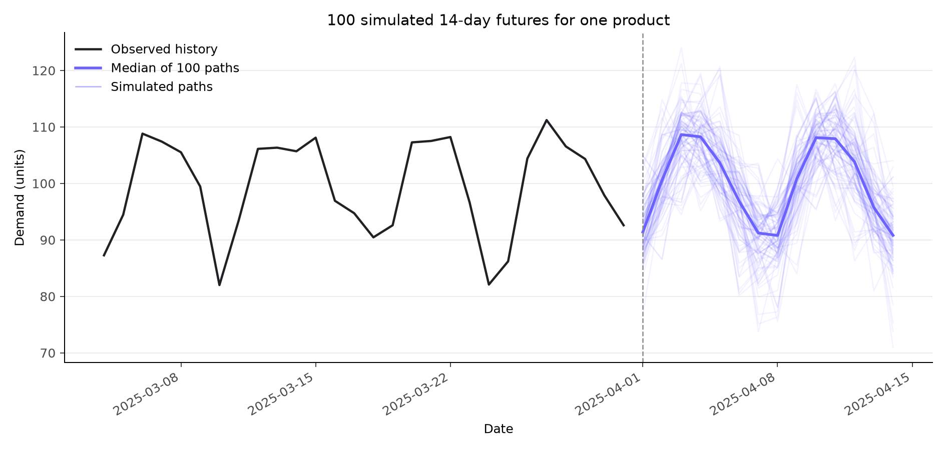 Each faint line is one complete, internally consistent future: the paths carry
the weekly rhythm forward and disagree about exactly how high the peaks and how
low the troughs will be. That disagreement is the uncertainty the next step
turns into numbers.
### Step 5: Understand the Output
| Column | Meaning |
| ----------- | ---------------------------------------------------------------------------------- |
| `unique_id` | Series identifier. It is omitted when the input has no ID column, as here. |
| `ds` | Future timestamp. |
| `sample_id` | Zero-based path identifier. Rows with the same ID belong to one future trajectory. |
| `TimeGPT` | Simulated target value. |
| `coupled` | Whether cross-series coupling was applied to this request. |
The output is long-form and ordered by `sample_id`, then series, then forecast
timestamp. Select one complete trajectory with:
```python theme={null}
path_7 = paths.query("sample_id == 7")
```
The pivot from Step 4 gives the complementary wide view: one column per path,
one row per future day.
### Step 6: Answer Risk Questions
Because each `sample_id` is a complete future, questions about the whole horizon
become simple group-by operations. What is the chance that demand drops below 80
units on at least one of the 14 days?
```python theme={null}
worst_day = paths.groupby("sample_id")["TimeGPT"].min()
(worst_day < 80).mean()
```
```text theme={null}
0.11
```
In 11% of the simulated futures, at least one day falls below 80 units. And how
much total demand should you plan for?
```python theme={null}
totals = paths.groupby("sample_id")["TimeGPT"].sum()
totals.quantile([0.1, 0.5, 0.9]).round(1)
```
```text theme={null}
0.1 1386.0
0.5 1396.5
0.9 1410.2
```
Eighty percent of the simulated futures put the 14-day total between roughly
1,386 and 1,410 units. Neither number can be read off a per-timestamp quantile
forecast: both depend on how the days within one future relate to each other.
Congratulations! You have generated simulated future paths with TimeGPT and
turned them into probability and risk estimates.
## Going Further
Compare simulated futures under different input assumptions, using real
electricity-price data and future exogenous variables.
Simulate several related products together so each future describes the
whole group at once.
## Choose the Number of Paths
`n_paths` controls the number of trajectories generated per series.
* Use tens of paths for exploration and plotting.
* Use hundreds or thousands when estimating probabilities or tail outcomes.
* Increase the count until the decision statistic you care about becomes stable.
* Response size and local dataframe memory grow linearly with `n_paths`.
The accepted range is 1 to 10,000 paths. The overall size of a request is also
bounded, counting the marginal grid the service builds alongside the paths:
```text theme={null}
number of series * h * (n_paths + number of quantiles) <= 10,000,000
```
When you do not pass a [quantile grid](#quantile-grid), the quantile count is
the model's native one. For example, 500 series, a horizon of 20, and 500 paths
is well inside the limit; raising the horizon to 200 would exceed it.
## Reproduce a Simulation
Provide an integer `seed` when you need a repeatable result: two calls with the
same data, arguments, and seed return the same paths. Repeated calls without
`seed` can return different paths. Use a fixed seed in tests, audited analyses,
and reproducible reports. The seed must be between `-2**63` and `2**64 - 1`.
## Advanced Usage
Features known across the forecast horizon belong in `X_df`, using the same
layout as [forecasting with exogenous
variables](/forecasting/exogenous-variables/numeric_features):
```python theme={null}
paths = nixtla_client.simulate(
df=df_train, # history including the feature columns
X_df=X_df, # h future rows per series with the same features
h=48,
freq="h",
n_paths=500,
seed=42,
)
```
Each future feature must also appear in the historical `df`, and `X_df` must
contain exactly `h` rows per series. Changing the future feature values is how
you simulate different scenarios — see [Scenario Analysis with
Simulation](/forecasting/probabilistic/simulation_scenarios) for a complete
walkthrough.
Declare features unavailable in the future with `hist_exog_list`:
```python theme={null}
paths = nixtla_client.simulate(
df=df_with_features,
h=14,
freq="D",
n_paths=100,
hist_exog_list=["feature_without_future_values"],
seed=1,
)
```
List categorical columns explicitly with `categorical_exog_list`. Future-known
categorical features also need their future values in `X_df`:
```python theme={null}
df_categorical = df.assign(
day_type=np.where(df["ds"].dt.dayofweek < 5, "weekday", "weekend"),
)
future_dates = pd.date_range(df["ds"].max() + pd.Timedelta(days=1), periods=14, freq="D")
X_df_categorical = pd.DataFrame(
{
"ds": future_dates,
"day_type": np.where(future_dates.dayofweek < 5, "weekday", "weekend"),
}
)
paths = nixtla_client.simulate(
df=df_categorical,
X_df=X_df_categorical,
h=14,
freq="D",
n_paths=100,
categorical_exog_list=["day_type"],
seed=1,
)
```
See [categorical features](/forecasting/exogenous-variables/categorical_features)
for the complete data requirements.
Date-derived features use the same interface as forecasting:
```python theme={null}
paths = nixtla_client.simulate(
df=df,
h=14,
freq="D",
n_paths=100,
date_features=["dayofweek"],
date_features_to_one_hot=["dayofweek"],
seed=1,
)
```
Learn more in the [date features guide](/forecasting/exogenous-variables/date_features).
Pass the ID returned by `finetune()`:
```python theme={null}
model_id = nixtla_client.finetune(df=df, freq="D", finetune_steps=10)
paths = nixtla_client.simulate(
df=df,
h=14,
freq="D",
n_paths=100,
finetuned_model_id=model_id,
seed=1,
)
```
The requested base model must match the base model used for fine-tuning. See
[reusing fine-tuned models](/forecasting/fine-tuning/save_reuse_delete_finetuned_models)
for model lifecycle guidance.
`simulate()` preserves the input dataframe library:
```python theme={null}
import polars as pl
pl_paths = nixtla_client.simulate(
df=pl.from_pandas(df),
h=14,
freq="1d",
n_paths=100,
seed=1,
)
```
Distributed dataframes are not currently supported.
You can provide a strictly increasing grid of between 2 and 200 values inside
the open interval `(0, 1)`:
```python theme={null}
paths = nixtla_client.simulate(
df=df,
h=14,
freq="D",
n_paths=100,
quantiles=[0.05, 0.25, 0.5, 0.75, 0.95],
seed=1,
)
```
A denser grid can represent the marginal forecast distribution in greater
detail, but it also increases computation and memory use.
`quantiles` does not add columns to the returned dataframe. It refines the
marginal distribution the paths are drawn from, so the output stays
`sample_id`, `TimeGPT`, and `coupled`. Compute any quantiles you need from the
paths themselves, or use
[quantile forecasts](/forecasting/probabilistic/quantiles) when quantile
columns are what you are after.
A wide grid counts towards the
[request size limit](#choose-the-number-of-paths): `number of series * h *
(n_paths + len(quantiles))` may not exceed 10,000,000.
If the payload exceeds the request size limit, pass `num_partitions` to split
the series across several concurrent requests:
```python theme={null}
paths = nixtla_client.simulate(
df=many_series,
h=24,
freq="h",
n_paths=200,
num_partitions=4,
)
```
The results are stitched back together, so the returned dataframe is the same
shape as an unpartitioned call.
`num_partitions` cannot be combined with `multivariate=True`, because coupling
is computed across the series within a single request. Partitioning would
return uncoupled paths, so the call is rejected instead.
Each partition is also sent a distinct seed derived from `seed`, so partitions
never share their random draws and the call stays reproducible. A partitioned
call still returns different paths than an unpartitioned one for the same
`seed`. Every path is a valid draw; only the specific values differ.
## Troubleshooting
### The series is too short
Simulation requires enough valid history to estimate forecast uncertainty and
to construct complete trajectories. The required length depends on the model,
horizon, and exogenous configuration. Add more history or reduce `h`.
### Future exogenous data has the wrong shape
For every future-known feature, provide exactly `h` values per series in `X_df`.
The ID and timestamps must match the requested future grid.
### The response is too large
Reduce `n_paths`, `h`, or the number of series. Remember that a long dataframe
has one row for every series, path, and future timestamp. If the *request* is
too large instead, see [partitioning](#advanced-usage).
### A repeated call changed
Provide the same integer `seed` and keep all data and arguments identical.
Simulated paths represent plausible model-based futures. They are not guaranteed
outcomes, and their quality depends on the data, model, horizon, and assumptions.
Validate decision rules with historical backtesting before using them in
production.
Each faint line is one complete, internally consistent future: the paths carry
the weekly rhythm forward and disagree about exactly how high the peaks and how
low the troughs will be. That disagreement is the uncertainty the next step
turns into numbers.
### Step 5: Understand the Output
| Column | Meaning |
| ----------- | ---------------------------------------------------------------------------------- |
| `unique_id` | Series identifier. It is omitted when the input has no ID column, as here. |
| `ds` | Future timestamp. |
| `sample_id` | Zero-based path identifier. Rows with the same ID belong to one future trajectory. |
| `TimeGPT` | Simulated target value. |
| `coupled` | Whether cross-series coupling was applied to this request. |
The output is long-form and ordered by `sample_id`, then series, then forecast
timestamp. Select one complete trajectory with:
```python theme={null}
path_7 = paths.query("sample_id == 7")
```
The pivot from Step 4 gives the complementary wide view: one column per path,
one row per future day.
### Step 6: Answer Risk Questions
Because each `sample_id` is a complete future, questions about the whole horizon
become simple group-by operations. What is the chance that demand drops below 80
units on at least one of the 14 days?
```python theme={null}
worst_day = paths.groupby("sample_id")["TimeGPT"].min()
(worst_day < 80).mean()
```
```text theme={null}
0.11
```
In 11% of the simulated futures, at least one day falls below 80 units. And how
much total demand should you plan for?
```python theme={null}
totals = paths.groupby("sample_id")["TimeGPT"].sum()
totals.quantile([0.1, 0.5, 0.9]).round(1)
```
```text theme={null}
0.1 1386.0
0.5 1396.5
0.9 1410.2
```
Eighty percent of the simulated futures put the 14-day total between roughly
1,386 and 1,410 units. Neither number can be read off a per-timestamp quantile
forecast: both depend on how the days within one future relate to each other.
Congratulations! You have generated simulated future paths with TimeGPT and
turned them into probability and risk estimates.
## Going Further
Compare simulated futures under different input assumptions, using real
electricity-price data and future exogenous variables.
Simulate several related products together so each future describes the
whole group at once.
## Choose the Number of Paths
`n_paths` controls the number of trajectories generated per series.
* Use tens of paths for exploration and plotting.
* Use hundreds or thousands when estimating probabilities or tail outcomes.
* Increase the count until the decision statistic you care about becomes stable.
* Response size and local dataframe memory grow linearly with `n_paths`.
The accepted range is 1 to 10,000 paths. The overall size of a request is also
bounded, counting the marginal grid the service builds alongside the paths:
```text theme={null}
number of series * h * (n_paths + number of quantiles) <= 10,000,000
```
When you do not pass a [quantile grid](#quantile-grid), the quantile count is
the model's native one. For example, 500 series, a horizon of 20, and 500 paths
is well inside the limit; raising the horizon to 200 would exceed it.
## Reproduce a Simulation
Provide an integer `seed` when you need a repeatable result: two calls with the
same data, arguments, and seed return the same paths. Repeated calls without
`seed` can return different paths. Use a fixed seed in tests, audited analyses,
and reproducible reports. The seed must be between `-2**63` and `2**64 - 1`.
## Advanced Usage
Features known across the forecast horizon belong in `X_df`, using the same
layout as [forecasting with exogenous
variables](/forecasting/exogenous-variables/numeric_features):
```python theme={null}
paths = nixtla_client.simulate(
df=df_train, # history including the feature columns
X_df=X_df, # h future rows per series with the same features
h=48,
freq="h",
n_paths=500,
seed=42,
)
```
Each future feature must also appear in the historical `df`, and `X_df` must
contain exactly `h` rows per series. Changing the future feature values is how
you simulate different scenarios — see [Scenario Analysis with
Simulation](/forecasting/probabilistic/simulation_scenarios) for a complete
walkthrough.
Declare features unavailable in the future with `hist_exog_list`:
```python theme={null}
paths = nixtla_client.simulate(
df=df_with_features,
h=14,
freq="D",
n_paths=100,
hist_exog_list=["feature_without_future_values"],
seed=1,
)
```
List categorical columns explicitly with `categorical_exog_list`. Future-known
categorical features also need their future values in `X_df`:
```python theme={null}
df_categorical = df.assign(
day_type=np.where(df["ds"].dt.dayofweek < 5, "weekday", "weekend"),
)
future_dates = pd.date_range(df["ds"].max() + pd.Timedelta(days=1), periods=14, freq="D")
X_df_categorical = pd.DataFrame(
{
"ds": future_dates,
"day_type": np.where(future_dates.dayofweek < 5, "weekday", "weekend"),
}
)
paths = nixtla_client.simulate(
df=df_categorical,
X_df=X_df_categorical,
h=14,
freq="D",
n_paths=100,
categorical_exog_list=["day_type"],
seed=1,
)
```
See [categorical features](/forecasting/exogenous-variables/categorical_features)
for the complete data requirements.
Date-derived features use the same interface as forecasting:
```python theme={null}
paths = nixtla_client.simulate(
df=df,
h=14,
freq="D",
n_paths=100,
date_features=["dayofweek"],
date_features_to_one_hot=["dayofweek"],
seed=1,
)
```
Learn more in the [date features guide](/forecasting/exogenous-variables/date_features).
Pass the ID returned by `finetune()`:
```python theme={null}
model_id = nixtla_client.finetune(df=df, freq="D", finetune_steps=10)
paths = nixtla_client.simulate(
df=df,
h=14,
freq="D",
n_paths=100,
finetuned_model_id=model_id,
seed=1,
)
```
The requested base model must match the base model used for fine-tuning. See
[reusing fine-tuned models](/forecasting/fine-tuning/save_reuse_delete_finetuned_models)
for model lifecycle guidance.
`simulate()` preserves the input dataframe library:
```python theme={null}
import polars as pl
pl_paths = nixtla_client.simulate(
df=pl.from_pandas(df),
h=14,
freq="1d",
n_paths=100,
seed=1,
)
```
Distributed dataframes are not currently supported.
You can provide a strictly increasing grid of between 2 and 200 values inside
the open interval `(0, 1)`:
```python theme={null}
paths = nixtla_client.simulate(
df=df,
h=14,
freq="D",
n_paths=100,
quantiles=[0.05, 0.25, 0.5, 0.75, 0.95],
seed=1,
)
```
A denser grid can represent the marginal forecast distribution in greater
detail, but it also increases computation and memory use.
`quantiles` does not add columns to the returned dataframe. It refines the
marginal distribution the paths are drawn from, so the output stays
`sample_id`, `TimeGPT`, and `coupled`. Compute any quantiles you need from the
paths themselves, or use
[quantile forecasts](/forecasting/probabilistic/quantiles) when quantile
columns are what you are after.
A wide grid counts towards the
[request size limit](#choose-the-number-of-paths): `number of series * h *
(n_paths + len(quantiles))` may not exceed 10,000,000.
If the payload exceeds the request size limit, pass `num_partitions` to split
the series across several concurrent requests:
```python theme={null}
paths = nixtla_client.simulate(
df=many_series,
h=24,
freq="h",
n_paths=200,
num_partitions=4,
)
```
The results are stitched back together, so the returned dataframe is the same
shape as an unpartitioned call.
`num_partitions` cannot be combined with `multivariate=True`, because coupling
is computed across the series within a single request. Partitioning would
return uncoupled paths, so the call is rejected instead.
Each partition is also sent a distinct seed derived from `seed`, so partitions
never share their random draws and the call stays reproducible. A partitioned
call still returns different paths than an unpartitioned one for the same
`seed`. Every path is a valid draw; only the specific values differ.
## Troubleshooting
### The series is too short
Simulation requires enough valid history to estimate forecast uncertainty and
to construct complete trajectories. The required length depends on the model,
horizon, and exogenous configuration. Add more history or reduce `h`.
### Future exogenous data has the wrong shape
For every future-known feature, provide exactly `h` values per series in `X_df`.
The ID and timestamps must match the requested future grid.
### The response is too large
Reduce `n_paths`, `h`, or the number of series. Remember that a long dataframe
has one row for every series, path, and future timestamp. If the *request* is
too large instead, see [partitioning](#advanced-usage).
### A repeated call changed
Provide the same integer `seed` and keep all data and arguments identical.
Simulated paths represent plausible model-based futures. They are not guaranteed
outcomes, and their quality depends on the data, model, horizon, and assumptions.
Validate decision rules with historical backtesting before using them in
production.