> ## Documentation Index
> Fetch the complete documentation index at: https://nixtla-docs-feat-simulate-and-explain.mintlify.site/llms.txt
> Use this file to discover all available pages before exploring further.
# Scenario Analysis with Simulation
> Compare simulated futures under different input assumptions, using real electricity-price data and future exogenous variables.
Scenario analysis asks: how does the range of possible futures change when the
inputs change? Simulation answers it by generating a full set of future paths
under each assumption, so you can compare complete outcome distributions rather
than two single forecasts.
This tutorial assumes you have seen the
[simulation quickstart](/forecasting/probabilistic/simulation). It walks
through a real energy-market question, then shows how to simulate several
series together as one coherent scenario.
## Real-data walkthrough: German electricity prices
This example uses the German electricity-price data from [Improve Forecast
Accuracy with TimeGPT](/forecasting/improve_accuracy). The target is the hourly
electricity price in EUR/MWh. The future inputs are published load and
generation forecasts — the kind of forward-looking information that belongs in
`X_df`.
### Step 1: Load the Data
```python theme={null}
import numpy as np
import pandas as pd
from nixtla import NixtlaClient
nixtla_client = NixtlaClient(
# Defaults to os.environ["NIXTLA_API_KEY"]
api_key="my_api_key_provided_by_nixtla"
)
data_url = (
"https://raw.githubusercontent.com/Nixtla/"
"transfer-learning-time-series/main/datasets/"
"electricity-short-with-ex-vars.csv"
)
energy = pd.read_csv(data_url, parse_dates=["ds"])
germany = energy.query('unique_id == "DE"').copy()
df_train = germany.query('ds < "2017-12-29"').copy()
df_test = germany.query('ds >= "2017-12-29"').copy()
X_df = df_test.drop(columns="y")
```
The final 48 hours are held out. In a live forecast, their prices would still
be unknown; here they let us compare the simulated futures with what was later
observed.
### Step 2: Simulate the Published-Input Scenario
Generate 500 possible 48-hour price paths using the published load and
generation forecasts:
```python theme={null}
paths = nixtla_client.simulate(
df=df_train,
X_df=X_df,
h=48,
freq="h",
n_paths=500,
seed=42,
model="timegpt-2.1",
)
paths.head()
```
| unique\_id | ds | sample\_id | TimeGPT | coupled |
| ---------- | ---------------- | ---------: | ------: | ------- |
| DE | 2017-12-29 00:00 | 0 | 12.30 | false |
| DE | 2017-12-29 01:00 | 0 | 9.71 | false |
| DE | 2017-12-29 02:00 | 0 | 7.99 | false |
| DE | 2017-12-29 03:00 | 0 | 7.38 | false |
| DE | 2017-12-29 04:00 | 0 | 10.01 | false |
The result contains `1 * 500 * 48 = 24,000` rows. Rows sharing a `sample_id`
form one complete electricity-price trajectory.
### Step 3: Simulate a Changed-Input Scenario
An energy buyer wants to understand what happens if system conditions tighten
on the second day. Create a scenario with:
* Load forecast 15% higher
* Generation forecast 15% lower
The first day remains unchanged, making the shift easy to see.
```python theme={null}
stress_X_df = X_df.copy()
stress_hours = (
stress_X_df["ds"].dt.date
== stress_X_df["ds"].dt.date.max()
)
stress_X_df.loc[stress_hours, "Exogenous1"] *= 1.15
stress_X_df.loc[stress_hours, "Exogenous2"] *= 0.85
stress_paths = nixtla_client.simulate(
df=df_train,
X_df=stress_X_df,
h=48,
freq="h",
n_paths=500,
seed=42,
model="timegpt-2.1",
)
```
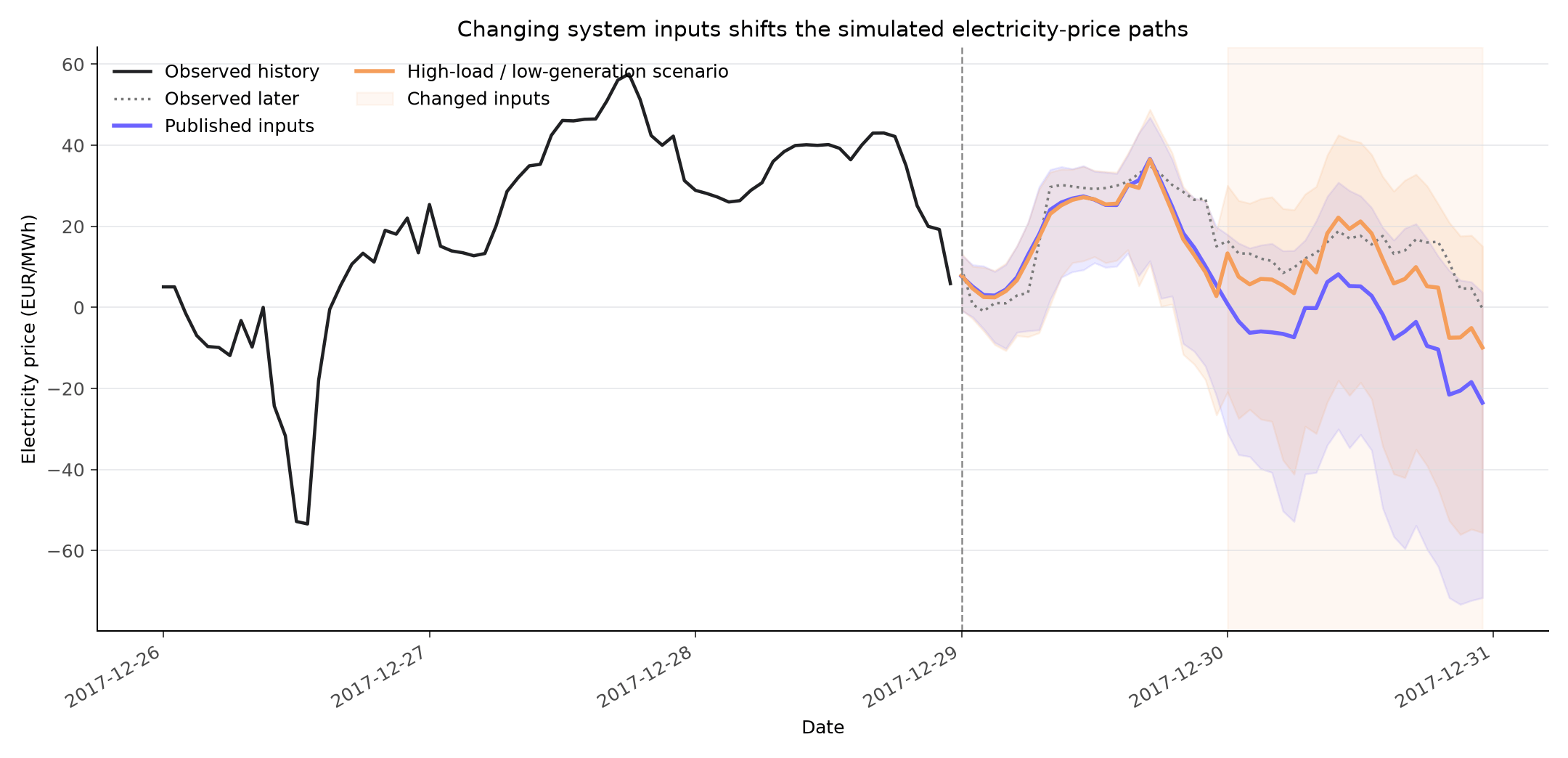 The scenarios overlap during the unchanged first day. During the changed second
day, the median stress path is **EUR 8.82 to EUR 16.02/MWh higher** than the
published-input path. New input assumptions produce a clearly different set of
future paths.
### Step 4: Convert the Paths into an Energy-Cost Risk
Suppose the buyer needs 1 MWh in every forecast hour. Summing each complete path
gives one possible 48-hour procurement cost:
```python theme={null}
baseline_cost = (
paths.groupby("sample_id", observed=True)["TimeGPT"]
.sum()
.rename("published_inputs")
)
stress_cost = (
stress_paths.groupby("sample_id", observed=True)["TimeGPT"]
.sum()
.rename("changed_inputs")
)
cost_summary = pd.DataFrame(
{
"Published inputs": [
baseline_cost.median(),
baseline_cost.quantile(0.9),
(baseline_cost > 300).mean(),
],
"Changed inputs": [
stress_cost.median(),
stress_cost.quantile(0.9),
(stress_cost > 300).mean(),
],
},
index=["Median cost", "90th percentile cost", "Probability above EUR 300"],
)
```
| 48-hour outcome | Published inputs | Changed inputs |
| ------------------------- | ---------------: | -------------: |
| Median cost | EUR 214.28 | EUR 509.86 |
| 90th percentile cost | EUR 840.23 | EUR 1,138.59 |
| Probability above EUR 300 | 43.0% | 67.0% |
The scenarios overlap during the unchanged first day. During the changed second
day, the median stress path is **EUR 8.82 to EUR 16.02/MWh higher** than the
published-input path. New input assumptions produce a clearly different set of
future paths.
### Step 4: Convert the Paths into an Energy-Cost Risk
Suppose the buyer needs 1 MWh in every forecast hour. Summing each complete path
gives one possible 48-hour procurement cost:
```python theme={null}
baseline_cost = (
paths.groupby("sample_id", observed=True)["TimeGPT"]
.sum()
.rename("published_inputs")
)
stress_cost = (
stress_paths.groupby("sample_id", observed=True)["TimeGPT"]
.sum()
.rename("changed_inputs")
)
cost_summary = pd.DataFrame(
{
"Published inputs": [
baseline_cost.median(),
baseline_cost.quantile(0.9),
(baseline_cost > 300).mean(),
],
"Changed inputs": [
stress_cost.median(),
stress_cost.quantile(0.9),
(stress_cost > 300).mean(),
],
},
index=["Median cost", "90th percentile cost", "Probability above EUR 300"],
)
```
| 48-hour outcome | Published inputs | Changed inputs |
| ------------------------- | ---------------: | -------------: |
| Median cost | EUR 214.28 | EUR 509.86 |
| 90th percentile cost | EUR 840.23 | EUR 1,138.59 |
| Probability above EUR 300 | 43.0% | 67.0% |
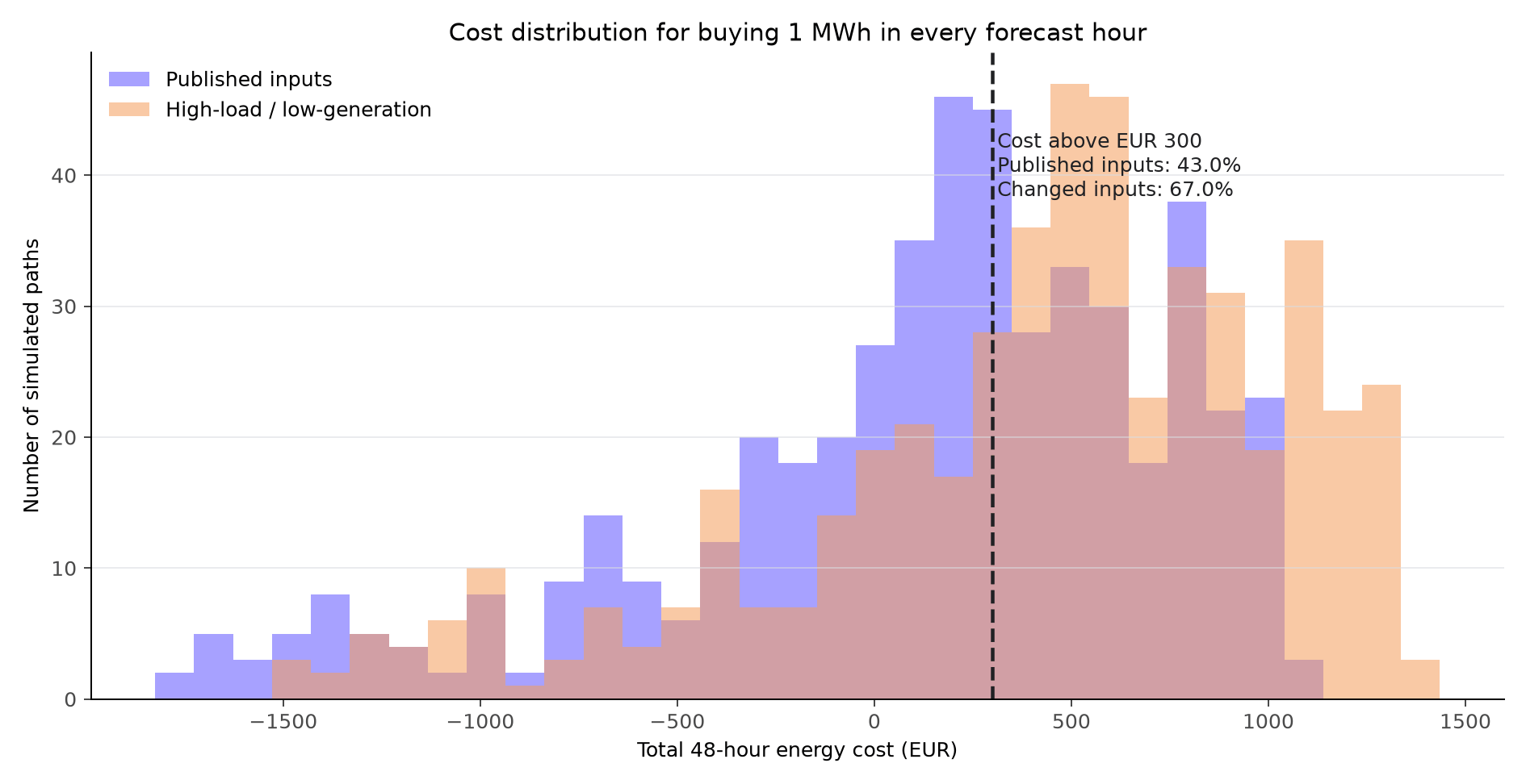 The changed system conditions do more than shift one hourly forecast: they move
the distribution of the complete purchasing outcome. A buyer can use this view
to compare a fixed-price offer, choose a hedge size, or set a budget buffer.
You have compared two complete outcome distributions under different input
assumptions — the core scenario-analysis workflow.
## Simulate Multiple Series Together
Pass stacked series using the normal `unique_id`, time, and target columns:
```python theme={null}
multi_df = energy.query(
'unique_id in ["BE", "FR"] and ds < "2016-12-29"'
)[
["unique_id", "ds", "y"]
]
market_paths = nixtla_client.simulate(
df=multi_df,
h=48,
freq="h",
n_paths=200,
seed=42,
)
```
By default, paths are generated independently for each series. Set
`multivariate=True` when each `sample_id` should represent one coherent scenario
across all series. This changes two things: the marginal forecasts become joint
for models that support it, so each series' distribution can reflect the others,
and the sample paths are coupled so that path `k` describes all series at once.
```python theme={null}
joint_paths = nixtla_client.simulate(
df=multi_df,
h=48,
freq="h",
n_paths=200,
seed=7,
multivariate=True,
)
joint_paths["coupled"].unique()
```
```text theme={null}
array([True])
```
Use a different `seed` when visually comparing coupled against uncoupled runs;
otherwise the first series can come back with identical paths in both, making
coupling look like it did nothing. Compare across-series statistics rather than
individual paths.
Both the coupled and the per-series shuffle draw from the same generator state,
so with a fixed seed the first series by ID is reordered identically whether
`multivariate` is True or False — and its paths come out the same whenever its
marginal forecast is unchanged too. Varying the seed removes this overlap from
visual comparisons.
The series must share a forecast origin. Different history lengths are allowed
because their common recent history is used. If the data does not contain a
shared, complete historical window, the request falls back to per-series paths
and returns `coupled=False`.
`coupled=False` is expected when `multivariate=False` or when the request
contains only one series. It does not indicate an error.
For a complete business example, see
[Plan Retail Promotions with Coupled Simulation](/use_cases/coupled_simulation_retail).
## Troubleshooting
### `coupled` is false
Check that:
* `multivariate=True`
* More than one series is present
* All series share the same forecast origin
* Their common recent history contains a complete window
Simulated paths represent plausible model-based futures. They are not guaranteed
outcomes, and their quality depends on the data, model, horizon, and assumptions.
Validate decision rules with historical backtesting before using them in
production.
The changed system conditions do more than shift one hourly forecast: they move
the distribution of the complete purchasing outcome. A buyer can use this view
to compare a fixed-price offer, choose a hedge size, or set a budget buffer.
You have compared two complete outcome distributions under different input
assumptions — the core scenario-analysis workflow.
## Simulate Multiple Series Together
Pass stacked series using the normal `unique_id`, time, and target columns:
```python theme={null}
multi_df = energy.query(
'unique_id in ["BE", "FR"] and ds < "2016-12-29"'
)[
["unique_id", "ds", "y"]
]
market_paths = nixtla_client.simulate(
df=multi_df,
h=48,
freq="h",
n_paths=200,
seed=42,
)
```
By default, paths are generated independently for each series. Set
`multivariate=True` when each `sample_id` should represent one coherent scenario
across all series. This changes two things: the marginal forecasts become joint
for models that support it, so each series' distribution can reflect the others,
and the sample paths are coupled so that path `k` describes all series at once.
```python theme={null}
joint_paths = nixtla_client.simulate(
df=multi_df,
h=48,
freq="h",
n_paths=200,
seed=7,
multivariate=True,
)
joint_paths["coupled"].unique()
```
```text theme={null}
array([True])
```
Use a different `seed` when visually comparing coupled against uncoupled runs;
otherwise the first series can come back with identical paths in both, making
coupling look like it did nothing. Compare across-series statistics rather than
individual paths.
Both the coupled and the per-series shuffle draw from the same generator state,
so with a fixed seed the first series by ID is reordered identically whether
`multivariate` is True or False — and its paths come out the same whenever its
marginal forecast is unchanged too. Varying the seed removes this overlap from
visual comparisons.
The series must share a forecast origin. Different history lengths are allowed
because their common recent history is used. If the data does not contain a
shared, complete historical window, the request falls back to per-series paths
and returns `coupled=False`.
`coupled=False` is expected when `multivariate=False` or when the request
contains only one series. It does not indicate an error.
For a complete business example, see
[Plan Retail Promotions with Coupled Simulation](/use_cases/coupled_simulation_retail).
## Troubleshooting
### `coupled` is false
Check that:
* `multivariate=True`
* More than one series is present
* All series share the same forecast origin
* Their common recent history contains a complete window
Simulated paths represent plausible model-based futures. They are not guaranteed
outcomes, and their quality depends on the data, model, horizon, and assumptions.
Validate decision rules with historical backtesting before using them in
production.