Scenario Analysis with Simulation

Scenario analysis asks: how does the range of possible futures change when the inputs change? Simulation answers it by generating a full set of future paths under each assumption, so you can compare complete outcome distributions rather than two single forecasts. This tutorial assumes you have seen the simulation quickstart. It walks through a real energy-market question, then shows how to simulate several series together as one coherent scenario.

Real-data walkthrough: German electricity prices

This example uses the German electricity-price data from Improve Forecast Accuracy with TimeGPT. The target is the hourly electricity price in EUR/MWh. The future inputs are published load and generation forecasts — the kind of forward-looking information that belongs in X_df.

Step 1: Load the Data

import numpy as np
import pandas as pd

from nixtla import NixtlaClient

nixtla_client = NixtlaClient(
    # Defaults to os.environ["NIXTLA_API_KEY"]
    api_key="my_api_key_provided_by_nixtla"
)

data_url = (
    "https://raw.githubusercontent.com/Nixtla/"
    "transfer-learning-time-series/main/datasets/"
    "electricity-short-with-ex-vars.csv"
)
energy = pd.read_csv(data_url, parse_dates=["ds"])
germany = energy.query('unique_id == "DE"').copy()

df_train = germany.query('ds < "2017-12-29"').copy()
df_test = germany.query('ds >= "2017-12-29"').copy()
X_df = df_test.drop(columns="y")

The final 48 hours are held out. In a live forecast, their prices would still be unknown; here they let us compare the simulated futures with what was later observed.

Step 2: Simulate the Published-Input Scenario

Generate 500 possible 48-hour price paths using the published load and generation forecasts:

paths = nixtla_client.simulate(
    df=df_train,
    X_df=X_df,
    h=48,
    freq="h",
    n_paths=500,
    seed=42,
    model="timegpt-2.1",
)

paths.head()

unique_id	ds	TimeGPT	coupled
DE	2017-12-29 00:00	12.30	false
DE	2017-12-29 01:00	9.71	false
DE	2017-12-29 02:00	7.99	false
DE	2017-12-29 03:00	7.38	false
DE	2017-12-29 04:00	10.01	false

The result contains 1 * 500 * 48 = 24,000 rows. Rows sharing a sample_id form one complete electricity-price trajectory.

Step 3: Simulate a Changed-Input Scenario

An energy buyer wants to understand what happens if system conditions tighten on the second day. Create a scenario with:

Load forecast 15% higher
Generation forecast 15% lower

The first day remains unchanged, making the shift easy to see.

stress_X_df = X_df.copy()
stress_hours = (
    stress_X_df["ds"].dt.date
    == stress_X_df["ds"].dt.date.max()
)

stress_X_df.loc[stress_hours, "Exogenous1"] *= 1.15
stress_X_df.loc[stress_hours, "Exogenous2"] *= 0.85

stress_paths = nixtla_client.simulate(
    df=df_train,
    X_df=stress_X_df,
    h=48,
    freq="h",
    n_paths=500,
    seed=42,
    model="timegpt-2.1",
)

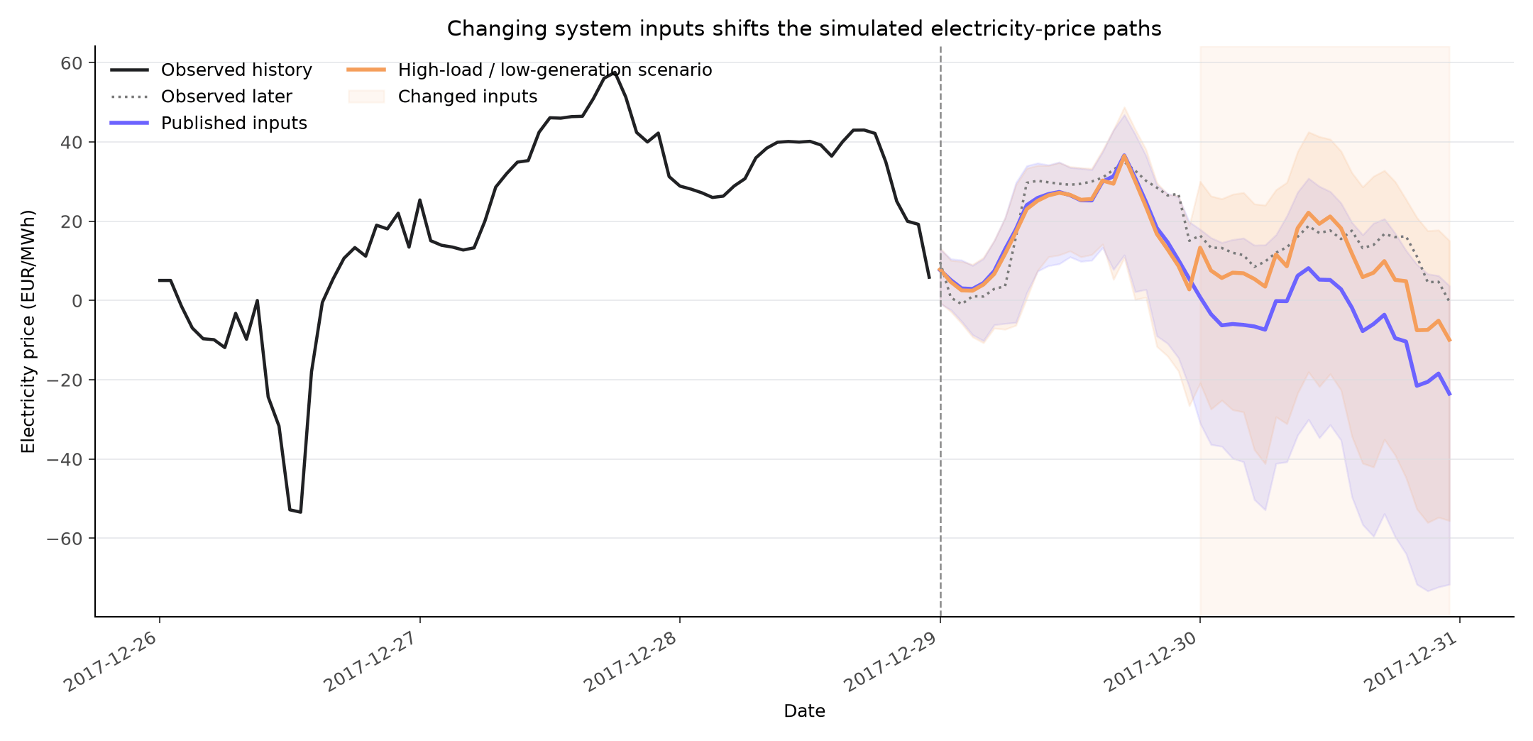
German electricity-price history and two simulated scenarios showing a clear upward shift after load rises and generation falls — Lines show the median path and shaded areas show the 10th–90th percentile range. The dotted line is the price observed after the forecast origin.

The scenarios overlap during the unchanged first day. During the changed second day, the median stress path is EUR 8.82 to EUR 16.02/MWh higher than the published-input path. New input assumptions produce a clearly different set of future paths.

Step 4: Convert the Paths into an Energy-Cost Risk

Suppose the buyer needs 1 MWh in every forecast hour. Summing each complete path gives one possible 48-hour procurement cost: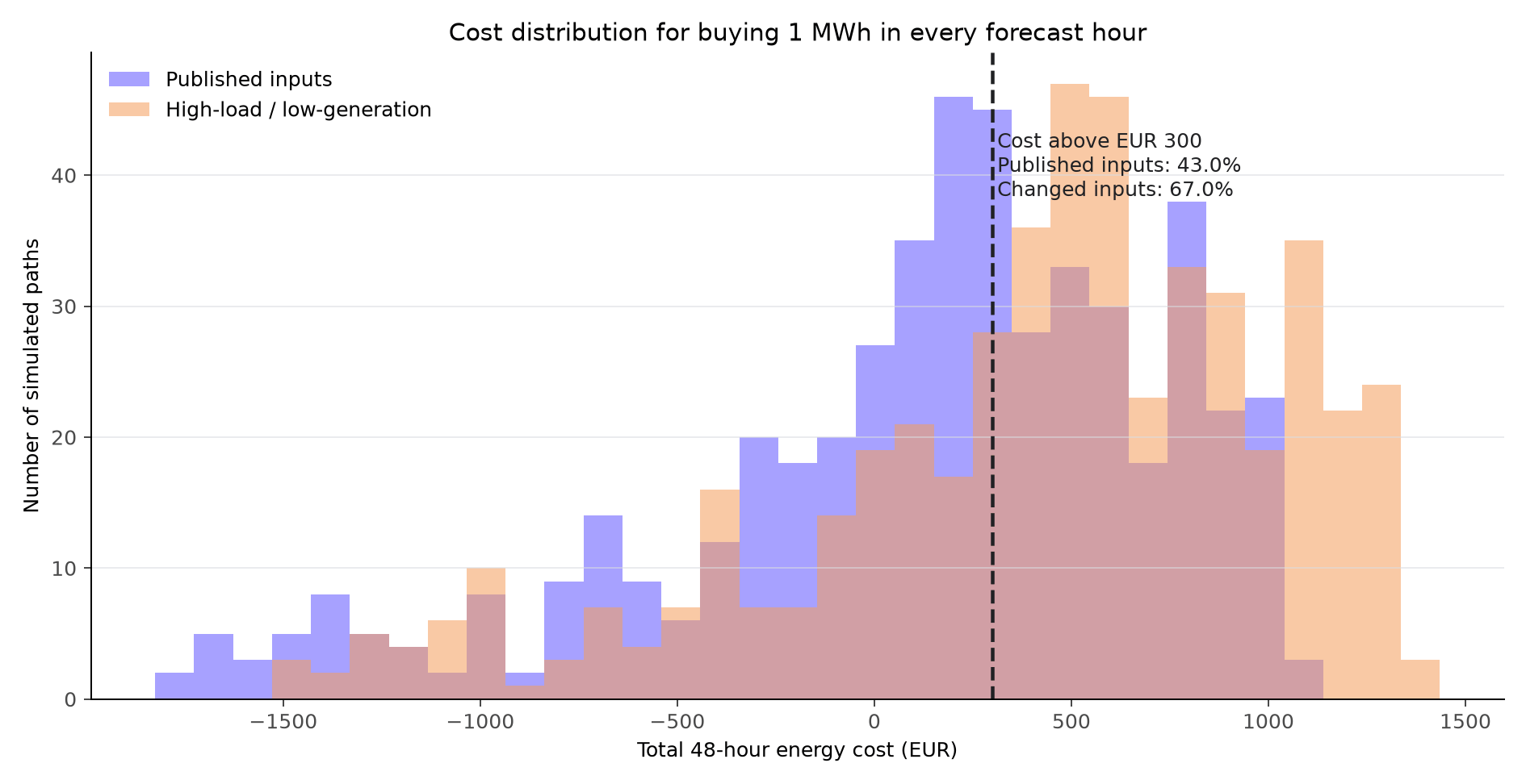

baseline_cost = (
    paths.groupby("sample_id", observed=True)["TimeGPT"]
    .sum()
    .rename("published_inputs")
)
stress_cost = (
    stress_paths.groupby("sample_id", observed=True)["TimeGPT"]
    .sum()
    .rename("changed_inputs")
)

cost_summary = pd.DataFrame(
    {
        "Published inputs": [
            baseline_cost.median(),
            baseline_cost.quantile(0.9),
            (baseline_cost > 300).mean(),
        ],
        "Changed inputs": [
            stress_cost.median(),
            stress_cost.quantile(0.9),
            (stress_cost > 300).mean(),
        ],
    },
    index=["Median cost", "90th percentile cost", "Probability above EUR 300"],
)

48-hour outcome	Published inputs	Changed inputs
Median cost	EUR 214.28	EUR 509.86
90th percentile cost	EUR 840.23	EUR 1,138.59
Probability above EUR 300	43.0%	67.0%

Overlapping histograms showing the higher 48-hour energy-cost distribution under changed inputs — Each observation is the total cost from one complete 48-hour path.

The changed system conditions do more than shift one hourly forecast: they move the distribution of the complete purchasing outcome. A buyer can use this view to compare a fixed-price offer, choose a hedge size, or set a budget buffer.

You have compared two complete outcome distributions under different input assumptions — the core scenario-analysis workflow.

Simulate Multiple Series Together

Pass stacked series using the normal unique_id, time, and target columns:

multi_df = energy.query(
    'unique_id in ["BE", "FR"] and ds < "2016-12-29"'
)[
    ["unique_id", "ds", "y"]
]

market_paths = nixtla_client.simulate(
    df=multi_df,
    h=48,
    freq="h",
    n_paths=200,
    seed=42,
)

By default, paths are generated independently for each series. Set multivariate=True when each sample_id should represent one coherent scenario across all series. This changes two things: the marginal forecasts become joint for models that support it, so each series’ distribution can reflect the others, and the sample paths are coupled so that path k describes all series at once.

joint_paths = nixtla_client.simulate(
    df=multi_df,
    h=48,
    freq="h",
    n_paths=200,
    seed=7,
    multivariate=True,
)

joint_paths["coupled"].unique()

array([True])

Use a different seed when visually comparing coupled against uncoupled runs; otherwise the first series can come back with identical paths in both, making coupling look like it did nothing. Compare across-series statistics rather than individual paths.

Why the seed matters when comparing runs

Both the coupled and the per-series shuffle draw from the same generator state, so with a fixed seed the first series by ID is reordered identically whether multivariate is True or False — and its paths come out the same whenever its marginal forecast is unchanged too. Varying the seed removes this overlap from visual comparisons.

The series must share a forecast origin. Different history lengths are allowed because their common recent history is used. If the data does not contain a shared, complete historical window, the request falls back to per-series paths and returns coupled=False.

coupled=False is expected when multivariate=False or when the request contains only one series. It does not indicate an error.

For a complete business example, see Plan Retail Promotions with Coupled Simulation.

Troubleshooting

`coupled` is false

Check that:

multivariate=True
More than one series is present
All series share the same forecast origin
Their common recent history contains a complete window

Simulated paths represent plausible model-based futures. They are not guaranteed outcomes, and their quality depends on the data, model, horizon, and assumptions. Validate decision rules with historical backtesting before using them in production.

INTRODUCTION

SETUP

DATA REQUIREMENTS

FORECASTING

ANOMALY DETECTION

USE CASES

REFERENCE

About

Real-data walkthrough: German electricity prices

Step 1: Load the Data

Step 2: Simulate the Published-Input Scenario

Step 3: Simulate a Changed-Input Scenario

Step 4: Convert the Paths into an Energy-Cost Risk

Simulate Multiple Series Together

Troubleshooting

`coupled` is false

​Real-data walkthrough: German electricity prices

​Step 1: Load the Data

​Step 2: Simulate the Published-Input Scenario

​Step 3: Simulate a Changed-Input Scenario

​Step 4: Convert the Paths into an Energy-Cost Risk

​Simulate Multiple Series Together

​Troubleshooting

​coupled is false

Real-data walkthrough: German electricity prices

Step 1: Load the Data

Step 2: Simulate the Published-Input Scenario

Step 3: Simulate a Changed-Input Scenario

Step 4: Convert the Paths into an Energy-Cost Risk

Simulate Multiple Series Together

Troubleshooting

`coupled` is false